Build a hydrological model

To get familiar with the HydroCNHS model construction process, let’s start with a hydrological model without human components. We will go through the following steps:

1. Create a model configuration file (.yaml) using a model builder.

2. Complete a model configuration file (.yaml)

3. Run a calibration

4. Run a simulation

We will adopt the following delineated watershed (Fig. 4) as a demonstration, in which we want to build a semi-distributed hydrological model to simulate the streamflow at the basin outlet, WSLO. The corresponding subbasins’ information is provided in Table 4.

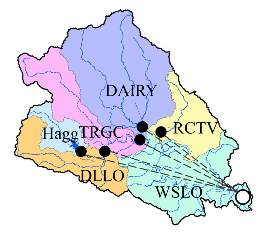
Fig. 4 Example watershed.

Table 4 Subbasins’ information.

Subbasin/outlet	Drainage area [ha]	Latitude [deg]	Flow length to WSLO [m]
Hagg	10034.2408	45.469	101469.139
DLLO	22568.2404	45.475	91813.075
TRGC	24044.6363	45.502	80064.864
DAIRY	59822.7546	45.520	70988.164
RCTV	19682.6046	45.502	60398.680
WSLO	47646.8477	45.350	0

Step 1: Create a model configuration file

HydroCNHS comes with a model builder to help users create an initial model configuration file.

First, initiate a model builder object with a working directory (your working folder directory).

import os
import HydroCNHS
prj_path, this_filename = os.path.split(__file__)

Second, set up the water system with the simulation period (i.e., start date and end date).

wd = prj_path
mb = HydroCNHS.ModelBuilder(wd)
mb.set_water_system(start_date="1981/1/1", end_date="2013/12/31")

Third, we can add subbasins (i.e., outlet_list) into the model. We adopt the GWLF model as the rainfall-runoff model (i.e., runoff_model). We also assign the corresponding subbasins’ areas (i.e., area_list) and latitude (i.e., lat_list) using the information from Table 4. Note that area_list and lat_list are optional arguments. Users can manually enter that information to the model configuration file (.yaml).

outlet_list = ['Hagg', 'DLLO', 'TRGC', 'DAIRY', 'RCTV', 'WSLO']
area_list = [10034.2408, 22568.2404, 24044.6363, 59822.7546, 19682.6046,
             47646.8477]
lat_list = [45.469, 45.475, 45.502, 45.520, 45.502, 45.350]
mb.set_rainfall_runoff(outlet_list=outlet_list,area_list=area_list,
                       lat_list=lat_list, runoff_model="GWLF")

Fourth, we want to add the routing setting. Here, we only have one routing outlet, WSLO, hence, we only need to run the following code once, and all the outlets are considered upstream outlets of WSLO.

flow_length_list = [101469.139, 91813.075, 80064.864, 70988.164, 60398.680, 0]
mb.set_routing_outlet(routing_outlet="WSLO",
                      upstream_outlet_list=outlet_list,
                      flow_length_list=flow_length_list)

Finally, we can print out the model for quick view and then write it to .yaml file with the given name.

### Print the model in the console
mb.print_model()

### Output initial model configuration file (.yaml)
mb.write_model_to_yaml(filename="HydroModel.yaml")

Now, we should have the initial model configuration file (i.e., HydroModel.yaml) in the corresponding folder.

Step 2: Complete a model configuration file

Before using the created HydroModel.yaml for the later experiment, we need to open it and ensure the information is correct. The “Inputs” in LSM and Routing sections should be all populated. Some default values may be used (e.g., \(S0\), \(U0\), and \(SnowS\)). They should be updated according to users’ needs. For this example, we don’t need to modify anything. You might notice that all the parameters have a value of -99. This is the default value in HydroCNHS, meaning that those values need to be calibrated if not provided by users.

Step 3: Run a calibration

First, we load the climate data, observed flow data at WSLO, and the model configuration file. Here, we have calculated the evapotranspiration using the Hamon method. Therefore, we load it as the inputs as well.

import matplotlib.pyplot as plt
import pandas as pd
import HydroCNHS.calibration as cali
from copy import deepcopy

# Load climate data
temp = pd.read_csv(os.path.join(wd,"Data","Temp_degC.csv"),
                index_col=["Date"]).to_dict(orient="list")
prec = pd.read_csv(os.path.join(wd,"Data","Prec_cm.csv"),
                index_col=["Date"]).to_dict(orient="list")
pet = pd.read_csv(os.path.join(wd,"Data","Pet_cm.csv"),
                index_col=["Date"]).to_dict(orient="list")

# Load flow gauge monthly data at WSLO
obv_flow_WSLO = pd.read_csv(os.path.join(wd,"Data","WSLO_M_cms.csv"),
                            index_col=["Date"], parse_dates=["Date"])

# Load model
model_dict = HydroCNHS.load_model(os.path.join(wd, "HydroModel.yaml"))

Second, we generate default parameter bounds and create a convertor for calibration. Details about the converter are provided in the Calibration section.

# Generate default parameter bounds
df_list, df_name = HydroCNHS.write_model_to_df(model_dict)
par_bound_df_list, df_name = HydroCNHS.gen_default_bounds(model_dict)

# Create convertor for calibration
converter = cali.Convertor()
cali_inputs = converter.gen_cali_inputs(wd, df_list, par_bound_df_list)
formatter = converter.formatter

Third, we program the evaluation function for a genetic algorithm (GA). Kling-Gupta efficiency (KGE; Gupta et al., 2009) is adopted to represent the model performance of simulated monthly streamflow at the WSLO routing outlet.

# Code evaluation function for GA algorthm
def evaluation(individual, info):
    cali_wd, current_generation, ith_individual, formatter, _ = info
    name = "{}-{}".format(current_generation, ith_individual)

    ##### individual -> model
    # Convert 1D array to a list of dataframes.
    df_list = cali.Convertor.to_df_list(individual, formatter)
    # Feed dataframes in df_list to model dictionary.
    model = deepcopy(model_dict)
    for i, df in enumerate(df_list):
        s = df_name[i].split("_")[0]
        model = HydroCNHS.load_df_to_model_dict(model, df, s, "Pars")

    ##### Run simuluation
    model = HydroCNHS.Model(model, name)
    Q = model.run(temp, prec, pet)

    ##### Get simulation data
    # Streamflow of routing outlets.
    cali_target = ["WSLO"]
    cali_period = ("1981-1-1", "2005-12-31")
    sim_Q_D = pd.DataFrame(Q, index=model.pd_date_index)[cali_target]
    # Resample the daily simulation output to monthly outputs.
    sim_Q_M = sim_Q_D[cali_target].resample("MS").mean()

    KGE = HydroCNHS.Indicator().KGE(
        x_obv=obv_flow_WSLO[cali_period[0]:cali_period[1]][cali_target],
        y_sim=sim_Q_M[cali_period[0]:cali_period[1]][cali_target])

    fitness = KGE
    return (fitness,)

Forth, we set up a GA for calibration. Again, we will explain calibration in more detail in the Calibration section. Here, the code is demonstrated. Note that calibration might take some time to run, depending on your system specifications. Users can lower down ‘pop_size ‘ and ‘max_gen’ if they just want to experience the process instead of seeking convergence. Note that to debug your code, please set ‘paral_cores’ to 1 to show the error messages.

config = {'min_or_max': 'max',
     'pop_size': 100,
     'num_ellite': 1,
     'prob_cross': 0.5,
     'prob_mut': 0.15,
     'stochastic': False,
     'max_gen': 100,
     'sampling_method': 'LHC',
     'drop_record': False,
     'paral_cores': -1,
     'paral_verbose': 1,
     'auto_save': True,
     'print_level': 1,
     'plot': True}

seed = 5
rn_gen = HydroCNHS.create_rn_gen(seed)
ga = cali.GA_DEAP(evaluation, rn_gen)
ga.set(cali_inputs, config, formatter, name="Cali_HydroModel_gwlf_KGE")
ga.run()
summary = ga.summary
individual = ga.solution

Finally, we export the calibrated model (i.e., Best_HydroModel_gwlf_KGE.yaml).

##### Output the calibrated model.
df_list = cali.Convertor.to_df_list(individual, formatter)
model_best = deepcopy(model_dict)
for i, df in enumerate(df_list):
    s = df_name[i].split("_")[0]
    model = HydroCNHS.load_df_to_model_dict(model_best, df, s, "Pars")
HydroCNHS.write_model(model_best, os.path.join(ga.cali_wd, "Best_HydroModel_gwlf_KGE.yaml"))

Step 4: Run a simulation

After obtaining a calibrated model, users can now use it for any simulation-based experiment (e.g., streamflow uncertainty under climate change). The calibrated model configuration file (e.g., Best_HydroModel_gwlf_KGE.yaml) can be directly loaded into HydroCNHS to run a simulation.

### Run a simulation.
model = HydroCNHS.Model(os.path.join(wd, "Cali_HydroModel_gwlf_KGE",
                                    "Best_HydroModel_gwlf_KGE.yaml"))
Q = model.run(temp, prec, pet)
result = pd.DataFrame(Q, index=model.pd_date_index).resample("MS").mean()

### Plot
fig, ax = plt.subplots()
ax.plot(obv_flow_WSLO.index, obv_flow_WSLO.loc[:, "WSLO"], label="Obv")
ax.plot(obv_flow_WSLO.index, result["WSLO"], ls="--", label="Sim")
ax.legend()

The complete script can be found at ./tutorials/Hydro_example/Main_HydroModel.py.

The following section will further introduce how to incorporate user-defined ABM modules into the model.