Integrate an ABM
After getting familiar with HydroCNHS from the hydrological model example in the previous section, we want to build a water system with human components (i.e., ABM). We will go through a similar process in the last example and focus on adding the human components.
Create a model configuration file (.yaml) using a model builder.
Complete a model configuration file (.yaml)
Program an ABM module (.py)
Run a calibration
Run a simulation
We adopt the Tualatin River Basin (TRB; Fig. 5; Table 5) as the tutorial example. The corresponding subbasins’ information is shown in Table 5. In this example, we consider three human components (Table 6), including (1) a reservoir (ResAgt), (2) an irrigation diversion (DivAgt), and (3) a trans-basin water transfer (PipeAgt), to demonstrate the HydroCNHS’s functionalities. Also, we model each human agent with different levels of behavioral complexities to provide users with a sense of how an agent can be modeled (Table 6). We will calibrate the model using the streamflow at DLLO and WSLO, reservoir releases from ResAgt, and water diversions from DivAgt on a monthly scale. More details about TRB can be found in Lin et al. (2022). Here, we focus on the coding part.
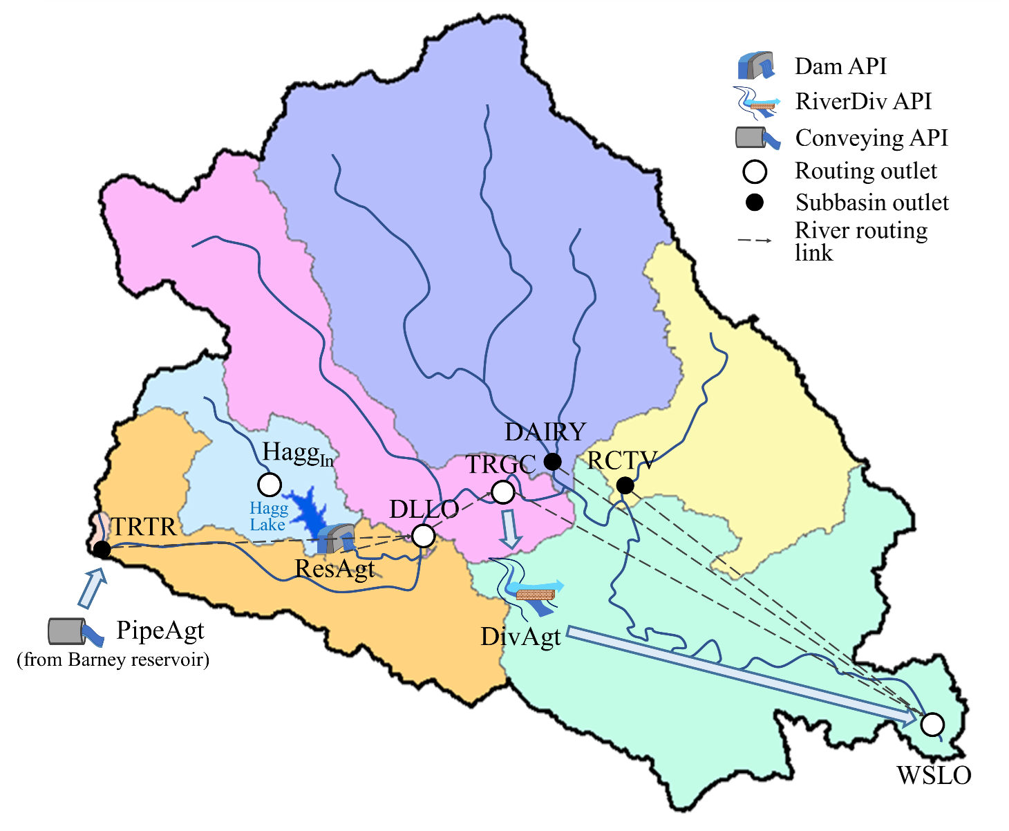
Fig. 5 The node-link structure of the Tualatin River Basin with human components.
Subbasin/outlet |
Drainage area [ha] |
Latitude [deg] |
Flow length [m] |
|---|---|---|---|
HaggIn |
10034.2408 |
45.469 |
0 (to HaggIn) |
TRTR |
329.8013 |
45.458 |
30899.4048 (to DLLO) |
ResAgt* |
– |
– |
9656.064 (to DLLO) |
DLLO |
22238.4391 |
45.475 |
0 (to DLLO)
11748.211 (to TRGC)
|
TRGC |
24044.6363 |
45.502 |
0 (to TRGC)
80064.864 (to WSLO)
|
DAIRY |
59822.7546 |
45.520 |
70988.164 (to WSLO) |
RCTV |
19682.6046 |
45.502 |
60398.680 (to WSLO) |
WSLO |
47646.8477 |
45.350 |
0 (to WSLO) |
*ResAgt is a reservoir agent integrated with Dam API. It is considered a pseudo routing outlet. |
|||
Item |
Agent name |
API |
Behavioral design |
From |
To |
|---|---|---|---|---|---|
Reservoir |
ResAgt |
Dam API |
Fixed operational rules |
HaggIn |
– |
Irrigation
diversion
|
DivAgt |
RiverDiv API |
Calibrated adaptive behavioral rules |
TRGC |
WSLO |
Trans-basin
water transfer
|
PipeAgt |
Conveying API |
External input data |
– |
TRTR |
Step 1: Create a model configuration file
Creating a node-link structure of a modeled water system is a vital step before using HydroCNHS. Subbasin outlets are determined based on the major tributaries in the TRB. However, the subbasin outlet, TRTR, is given because we have an inlet there for trans-basin water transfer. For the routing outlet assignment, DLLO and WSLO are selected because the streamflow at these two is part of the calibration targets, TRGC is also chosen since an agent integrated using RiverDiv API can only divert water from a routing outlet, and HaggIn is picked because it is the inflow of ResAgt (i.e., ResAgt takes water from HaggIn).
With a node-link structure of the TRB water system, we can follow the same process shown in the “Build a hydrological model” to initialize a model builder, set up the water system with the simulation period, add subbasins, and add four routing outlets. Note that ResAgt is considered a pseudo routing outlet that needs to be assigned to one of the upstream outlets of a routing outlet.
import os
import HydroCNHS
prj_path, this_filename = os.path.split(__file__)

### Initialize a model builder object.
wd = prj_path
mb = HydroCNHS.ModelBuilder(wd)

### Setup a water system simulation information
mb.set_water_system(start_date="1981/1/1", end_date="2013/12/31")

### Setup land surface model (rainfall-runoff model)
# Here we have seven subbasins and we select GWLF as the rainfall-runoff model.
outlet_list = ['HaggIn', 'TRTR', 'DLLO', 'TRGC', 'DAIRY', 'RCTV', 'WSLO']
area_list = [10034.2408, 329.8013, 22238.4391, 24044.6363, 59822.7546,
            19682.6046, 47646.8477]
lat_list = [45.469, 45.458, 45.475, 45.502, 45.520, 45.502, 45.350]
mb.set_rainfall_runoff(outlet_list=outlet_list,area_list=area_list,
                    lat_list=lat_list, runoff_model="GWLF")

### Setup routing outlets
# Add WSLO
mb.set_routing_outlet(routing_outlet="WSLO",
                    upstream_outlet_list=["TRGC", "DAIRY", "RCTV", "WSLO"],
                    flow_length_list=[80064.864, 70988.164, 60398.680, 0])
# Add TRGC
mb.set_routing_outlet(routing_outlet="TRGC",
                    upstream_outlet_list=["DLLO", "TRGC"],
                    flow_length_list=[11748.211, 0])
# Add DLLO
# Specify that ResAgt is an instream object.
mb.set_routing_outlet(routing_outlet="DLLO",
                    upstream_outlet_list=["ResAgt", "TRTR", "DLLO"],
                    flow_length_list=[9656.064, 30899.4048, 0],
                    instream_objects=["ResAgt"])
# Add HaggIn
mb.set_routing_outlet(routing_outlet="HaggIn",
                    upstream_outlet_list=["HaggIn"],
                    flow_length_list=[0])
Initialize ABM setting
To add human components, we need to first initialize the ABM setting block by assigning an ABM module folder’s directory and planned ABM module filename. If they are not given, default values will be applied, namely, working directory and “ABM_module.py, “respectively. abm_module_name will be used as the filename for the ABM module template if users choose to generate one using the model builder.
mb.set_ABM(abm_module_folder_path=wd, abm_module_name="TRB_ABM.py")
Add agents
Next, we add human components (i.e., agents) to the model builder. We first add a reservoir agent (ResAgt), in which its corresponding agent type class, agent name, api, link dictionary, and decision-making class can be assigned at this stage. Although not all information has to be provided now (i.e., it can be manually added to the model configuration file later), we encourage users to provide complete details here.
mb.add_agent(agt_type_class="Reservoir_AgtType", agt_name="ResAgt",
             api=mb.api.Dam,
             link_dict={"HaggIn": -1, "ResAgt": 1},
             dm_class="ReleaseDM")
The setting shown above means that ResAgt (an agent object) will be created from Reservoir_AgtType (an agent type class) and integrated into HydroCNHS using the Dam API. A decision-making object will be created from ReleaseDM (a decision-making class) and assigned to ResAgt as its attribute. This agent, ResAgt, will take water (factor = -1) from HaggIn routing outlet and release (factor = 1) water to ResAgt. Remember that ResAgt itself is a pseudo routing outlet.
Following a similar procedure, we add a water diversion agent (DivAgt). However, we have parameters, including ReturnFactor, a, and b, involved in this agent. Hence, a dictionary is provided to the par_dict argument. The format of the parameter dictionary is that keys are parameter names, and values are parameter values (-99 means waiting to be calibrated).
However, if the parameter is the factor used in the link_dict, users need to follow the format shown here. For example, we want to calibrate a return factor (ReturnFactor) to determine the portion of diverted water returned to the WSLO subbasin. To do that, a list, [“ReturnFactor”, 0, “Plus”], is given to link_dict at WSLO. HydroCNHS will interpret it as taking the factor value from parameter ReturnFactor with a list index of 0. “Plus” tells HydroCNHS we add water to WSLO. If water is taken from WSLO, then “Minus” should be assigned.
mb.add_agent(agt_type_class="Diversion_AgType", agt_name="DivAgt",
             api=mb.api.RiverDiv,
             link_dict={"TRGC": -1, "WSLO": ["ReturnFactor", 0, "Plus"]},
             dm_class="DivertDM",
             par_dict={"ReturnFactor": [-99], "a": -99, "b":-99})
Finally, we add a trans-basin water transfer agent (PipeAgt).
mb.add_agent(agt_type_class="Pipe_AgType", agt_name="PipeAgt",
             api=mb.api.Conveying,
             link_dict={"TRTR": 1},
             dm_class="TransferDM")
Add institution
We did not include an institution in this TRB example; however if users want to assign an institution (e.g., “ResDivInstitution”) to ResAgt and DivAgt, they should do so by assuming that there is a cooperation between water release decisions and water diversion decisions. Namely, release decisions from ResAgt and diversion decisions from DivAgt are made simultaneously using a single decision-making object (Fig. 6). Users can do the following.
mb.add_institution(institution="ResDivInstitution",
                   instit_dm_class=" ResDivDMClass",
                   agent_list=[" ResAgt ", "DivAgt"])
Note that ResDivInstitution will overwrite the originally assigned DM classes (if any) of ResAgt and DivAgt. The above command means a single ResDivInstitution decision-making object initialized from ResDivDMClass will be assigned to ResAgt and DivAgt’s attributes (e.g., self.dm). Users can utilize this property to design their agents.
Generate ABM module template & output model configuration file
In addition to outputting a model configuration file (.yaml), the model builder can generate an ABM module template (.py) for users, in which the model builder will create the outline of agent type classes and decision-making classes, and users can concentrate on programming the calculation for each class given in the template.
### Output initial model configuration file (.yaml) and ABM module template.
mb.write_model_to_yaml(filename="HydroABMModel.yaml")
mb.gen_ABM_module_template()
Step 2: Complete a model configuration file
After the model configuration file (.yaml) is created, users should open the file to complete and correct any missing or misinterpreted values. For this example, again, we will keep the default values.
Step 3: Program ABM module (.py)
In the generated ABM module (.py), users can find mainly two types of classes, including agent type classes (AgtType) and decision-making classes (DMClass/Institutional DMClass). Agent type classes are used to define agents’ actions and store up-to-date information (e.g., current date and current time step) in agents’ attributes. Decision-making classes are used to program a specific decision-making process. Decision-making classes can be further separated into DMClass and Institutional DMClass.
The ABM design logic is illustrated in Fig. 6. A “class” is a template for objects that can be initiated with object-specific attributes and settings. For example, Agent1 and Agent2 are initiated from the same AgtType1 class. Agent 2, Agent 4, and Agent 5 are initiated from the AgtType2 class. Each agent will be assigned a DM object or Institution object as one of its attributes. DM objects initiated from DMClass are NOT shared with other agents; Namely, agents with DM objects will only have one unique DM object (e.g., Agent 1 and Agent 2 in Fig. 6). In contrast, an Institution object can be shared with multiple agents, in which those agents can make decisions together. For example, multiple irrigation districts make diversion decisions together to share the water shortage during a drought period. We will not implement the Institutional DMClass in this TRB example; however, we will show how to add an institution through a model builder.
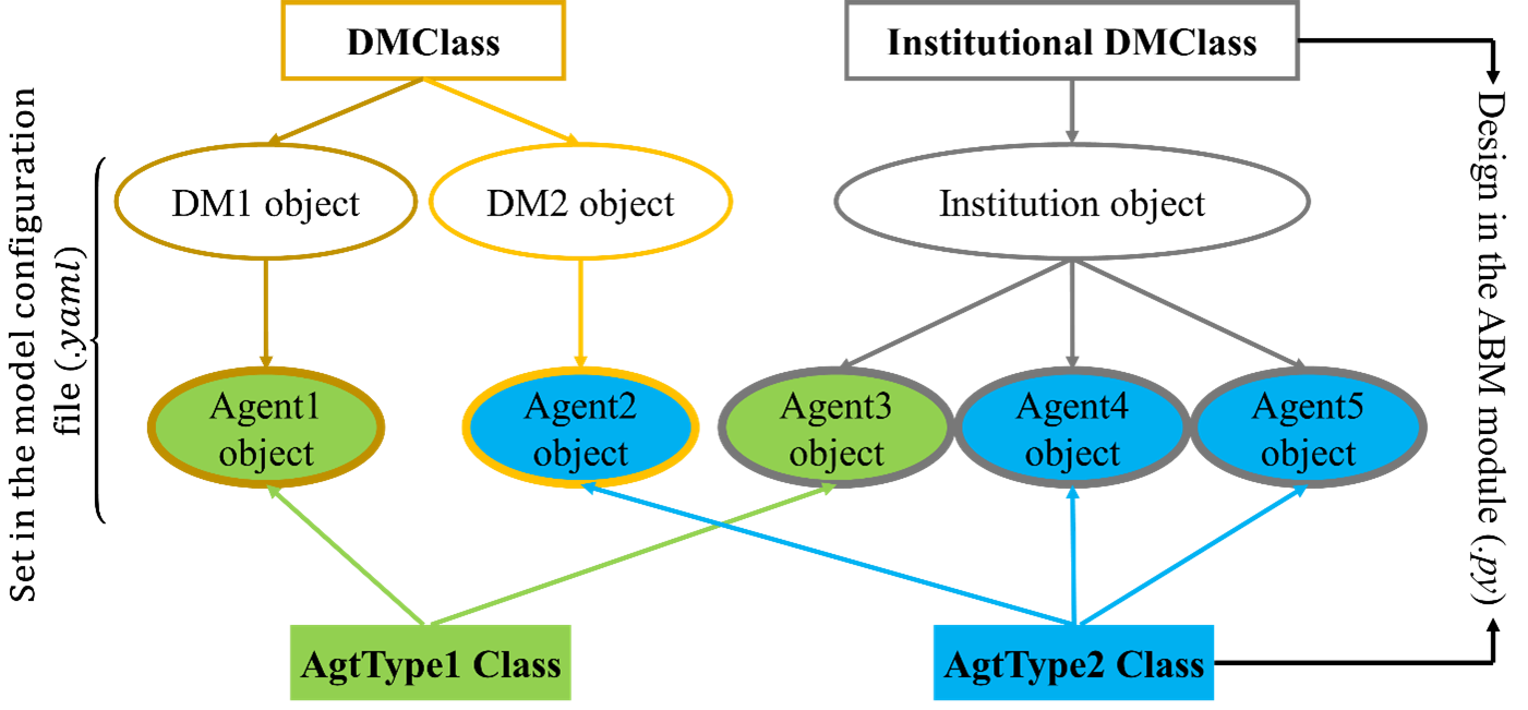
Fig. 6 ABM design logic. An agent is a combination of an AgtType class and an (Institutional) DM class. An Institution object can be shared among a group of agent objects (i.e., make decisions together), while a DM object can only be assigned to one agent object.
Agent type class (AgtType):
self.name = agent’s name
self.config = agent’s configuration dictionary, {‘Attributes’: …, ‘Inputs’: …, ‘Pars’: …}.
self.start_date = start date (datetime object).
self.current_date = current date (datetime object).
self.data_length = data/simulation length.
self.t = current timestep.
self.dc = data collector object containing data. Routed streamflow (Q_routed) is also collected here.
self.rn_gen = NumPy random number generator.
self.agents = a dictionary of all initialized agents, {agt_name: agt object}.
self.dm = (institutional) decision-making object if DMClass or institution is assigned to the agent, else None.
# AgtType
class XXX_AgtType(Base):
    def __init__(self, **kwargs):
        super().__init__(**kwargs)
        # The AgtType inherited attributes are applied.
        # See the note at top.

    def act(self, outlet):
        # Read corresponding factor of the given outlet
        factor = read_factor(self.config, outlet)

        # Common usage:
        # Get streamflow of outlet at timestep t
        Q = self.dc.Q_routed[outlet][self.t]

        # Make decision from (Institutional) decision-making
        # object if self.dm is not None.
        #decision = self.dm.make_dm(your_arguments)

        if factor <= 0:     # Divert from the outlet
            action = 0
        elif factor > 0:    # Add to the outlet
            action = 0

        return action
(Institutional) decision-making classes (DMClass):
self.name = name of the agent or institute.
self.dc = data collector object containing data. Routed streamflow (Q_routed) is also collected here.
self.rn_gen = NumPy random number generator.
# DMClass
class XXX_DM(Base):
    def __init__(self, **kwargs):
        super().__init__(**kwargs)
        # The (Institutional) DMClass inherited attributes are applied.
        # See the note at top.

    def make_dm(self, your_arguments):
        # Decision-making calculation.
        decision = None
        return decision
To keep the manual concise, we provide a complete ABM module for the TRB example at ./tutorials/HydroABM_example/TRB_ABM_complete.py. Theoretical details can be found in Lin et al. (2022), and more coding tips are available at Advanced ABM coding tips.
Step 4: Run a calibration
First, we load the model configuration file, the climate data, and the observed monthly flow data for DLLO and WSLO, reservoir releases of ResAgt, and water diversions of DivAgt. Here, we have calculated the evapotranspiration using the Hamon method. Therefore, PET data is input along with other data. Note that we manually change the ABM module from “TRB_ABM.py” to “TRB_ABM_complete.py.”
import matplotlib.pyplot as plt
import pandas as pd
import HydroCNHS.calibration as cali
from copy import deepcopy

# Load climate data
temp = pd.read_csv(os.path.join(wd,"Data","Temp_degC.csv"),
                index_col=["Date"]).to_dict(orient="list")
prec = pd.read_csv(os.path.join(wd,"Data","Prec_cm.csv"),
                index_col=["Date"]).to_dict(orient="list")
pet = pd.read_csv(os.path.join(wd,"Data","Pet_cm.csv"),
                index_col=["Date"]).to_dict(orient="list")

# Load flow gauge monthly data at WSLO
obv_flow_data = pd.read_csv(os.path.join(wd,"Data","Cali_M_cms.csv"),
                            index_col=["Date"], parse_dates=["Date"])

# Load model
model_dict = HydroCNHS.load_model(os.path.join(wd, "HydroABMModel.yaml"))
# Change the ABM module to the complete one.
model_dict["WaterSystem"]["ABM"]["Modules"] = ["TRB_ABM_complete.py"]
Second, we generate default parameter bounds and create a convertor for calibration. Note that we manually change the default ABM parameter bounds as shown in the code. Details about the Converter are provided in the Calibration section.
# Generate default parameter bounds
df_list, df_name = HydroCNHS.write_model_to_df(model_dict)
par_bound_df_list, df_name = HydroCNHS.gen_default_bounds(model_dict)

# Modify the default bounds of ABM
df_abm_bound = par_bound_df_list[2]
df_abm_bound.loc["ReturnFactor.0", [('DivAgt', 'Diversion_AgType')]] = "[0, 0.5]"
df_abm_bound.loc["a", [('DivAgt', 'Diversion_AgType')]] = "[-1, 1]"
df_abm_bound.loc["b", [('DivAgt', 'Diversion_AgType')]] = "[-1, 1]"

# Create convertor for calibration
converter = cali.Convertor()
cali_inputs = converter.gen_cali_inputs(wd, df_list, par_bound_df_list)
formatter = converter.formatter
Third, we program the evaluation function for a genetic algorithm (GA). The four calibration targets’ mean Kling-Gupta efficiency (KGE; Gupta et al., 2009) is adopted to represent the model performance.
# Code evaluation function for GA algorthm
def evaluation(individual, info):
    cali_wd, current_generation, ith_individual, formatter, _ = info
    name = "{}-{}".format(current_generation, ith_individual)

    ##### individual -> model
    # Convert 1D array to a list of dataframes.
    df_list = cali.Convertor.to_df_list(individual, formatter)
    # Feed dataframes in df_list to model dictionary.
    model = deepcopy(model_dict)
    for i, df in enumerate(df_list):
        s = df_name[i].split("_")[0]
        model = HydroCNHS.load_df_to_model_dict(model, df, s, "Pars")

    ##### Run simuluation
    model = HydroCNHS.Model(model, name)
    Q = model.run(temp, prec, pet)

    ##### Get simulation data
    # Streamflow of routing outlets.
    cali_target = ["WSLO","DLLO","ResAgt","DivAgt"]
    cali_period = ("1981-1-1", "2005-12-31")
    sim_Q_D = pd.DataFrame(Q, index=model.pd_date_index)[["WSLO","DLLO"]]
    sim_Q_D["ResAgt"] = model.dc.ResAgt["Release"]
    sim_Q_D["DivAgt"] = model.dc.DivAgt["Diversion"]
    # Resample the daily simulation output to monthly outputs.
    sim_Q_M = sim_Q_D[cali_target].resample("MS").mean()

    KGEs = []
    for target in cali_target:
        KGEs.append(HydroCNHS.Indicator().KGE(
            x_obv=obv_flow_data[cali_period[0]:cali_period[1]][[target]],
            y_sim=sim_Q_M[cali_period[0]:cali_period[1]][[target]]))

    fitness = sum(KGEs)/4
    return (fitness,)
Fourth, we set up a GA for calibration. Again, we will explain calibration in more detail in the Calibration section. Here, only the code is demonstrated. Note that calibration might take some time to run, depending on your system specifications. Users can lower down ‘pop_size’ and ‘max_gen’ if they want to experience the process instead of seeking convergence. In order to debug your code, set ‘paral_cores’ to 1 to show the error message.
config = {'min_or_max': 'max',
        'pop_size': 100,
        'num_ellite': 1,
        'prob_cross': 0.5,
        'prob_mut': 0.15,
        'stochastic': False,
        'max_gen': 100,
        'sampling_method': 'LHC',
        'drop_record': False,
        'paral_cores': -1,
        'paral_verbose': 1,
        'auto_save': True,
        'print_level': 1,
        'plot': True}

seed = 5
rn_gen = HydroCNHS.create_rn_gen(seed)
ga = cali.GA_DEAP(evaluation, rn_gen)
ga.set(cali_inputs, config, formatter, name="Cali_HydroABMModel_gwlf_KGE")
ga.run()
summary = ga.summary
individual = ga.solution
Finally, we export the calibrated model (i.e., Best_HydroABMModel_gwlf_KGE.yaml).
##### Output the calibrated model.
df_list = cali.Convertor.to_df_list(individual, formatter)
model_best = deepcopy(model_dict)
for i, df in enumerate(df_list):
    s = df_name[i].split("_")[0]
    model = HydroCNHS.load_df_to_model_dict(model_best, df, s, "Pars")
HydroCNHS.write_model(model_best, os.path.join(ga.cali_wd, "Best_HydroABMModel_gwlf_KGE.yaml"))
Step 5: Run a simulation
After obtaining a calibrated model, users can now use it for any simulation-based experiment (e.g., streamflow uncertainty under climate change). The calibrated model configuration file (i.e., Best_HydroABMModel_gwlf_KGE.yaml) can be directly loaded into HydroCNHS to run a simulation.
### Run a simulation.
model = HydroCNHS.Model(os.path.join(ga.cali_wd, "Best_HydroABMModel_gwlf_KGE.yaml"))
Q = model.run(temp, prec, pet)
sim_Q_D = pd.DataFrame(Q, index=model.pd_date_index)[["WSLO","DLLO"]]
sim_Q_D["ResAgt"] = model.dc.ResAgt["Release"]
sim_Q_D["DivAgt"] = model.dc.DivAgt["Diversion"]
sim_Q_M = sim_Q_D[["WSLO","DLLO","ResAgt","DivAgt"]].resample("MS").mean()
### Plot
fig, axes = plt.subplots(nrows=4, sharex=True)
axes = axes.flatten()
x = sim_Q_M.index
axes[0].plot(x, sim_Q_M["DLLO"], label="$M_{gwlf}$")
axes[1].plot(x, sim_Q_M["WSLO"], label="$M_{gwlf}$")
axes[2].plot(x, sim_Q_M["ResAgt"], label="$M_{gwlf}$")
axes[3].plot(x, sim_Q_M["DivAgt"], label="$M_{gwlf}$")

axes[0].plot(x, obv_flow_data["DLLO"], ls="--", lw=1, color="black", label="Obv")
axes[1].plot(x, obv_flow_data["WSLO"], ls="--", lw=1, color="black", label="Obv")
axes[2].plot(x, obv_flow_data["ResAgt"], ls="--", lw=1, color="black", label="Obv")
axes[3].plot(x, obv_flow_data["DivAgt"], ls="--", lw=1, color="black", label="Obv")

axes[0].set_ylim([0,75])
axes[1].set_ylim([0,230])
axes[2].set_ylim([0,23])
axes[3].set_ylim([0,2])

axes[0].set_ylabel("DLLO\n($m^3/s$)")
axes[1].set_ylabel("WSLO\n($m^3/s$)")
axes[2].set_ylabel("Release\n($m^3/s$)")
axes[3].set_ylabel("Diversion\n($m^3/s$)")

axes[0].axvline(pd.to_datetime("2006-1-1"), color="grey", ls="-", lw=1)
axes[1].axvline(pd.to_datetime("2006-1-1"), color="grey", ls="-", lw=1)
axes[2].axvline(pd.to_datetime("2006-1-1"), color="grey", ls="-", lw=1)
axes[3].axvline(pd.to_datetime("2006-1-1"), color="grey", ls="-", lw=1)

axes[0].legend(ncol=3, bbox_to_anchor=(1, 1.5), fontsize=9)

fig.align_ylabels(axes)